In the second part of this project, we will carry out exploratory data analysis on the data we collected in part 1. This EDA part consists of two main sections: organising and preparing the dataframes for visualisation using Pandas, and data visualisation using Pandas and Plotly. The main goal of this analysis is to find out if swimmers are faster in the water (excluding the reaction time) during relays than during individual races, and if yes, what are the factors influencing faster relay “time in water”. In the first section, we calculate our binary dependent variable (whether a swimmer’s “time in water” was faster in the relay leg or the individual event) and organise the data that we scraped to have as many explanatory variables to test as possible. In the second section, we study the individual and grouped effect of those explanatory variables on our main dependent variable and visualise the results with many different kinds of plots: tornado graphs, scatter plots, histograms, and box plots. Given that the data sampling carried out in the first part was not random (time bound), the reader should bear in mind that the insights obtained in this exploratory data analysis cannot be generalised to accurately describe the entire population, nor can they accurately predict future performances.
Data preparation: organising the data for visualisation
# imports and defining constants
from sqlalchemy import create_engine
import pandas as pd
import numpy as np
import statsmodels.api as sm
from datetime import datetime as dt
import plotly.graph_objects as go
import plotly.express as px
TIME_FORMAT_LONG = "%M:%S.%f"
TIME_FORMAT_SHORT = "%S.%f"
Preliminary step: importing data from the database & how to interpret the results of this EDA
We first import the data from an SQLite database file, and make several important remarks to better understand how we will interpret the results of the data analysis in the next section:
engine = create_engine("sqlite+pysqlite:///major_meets_2015-2023.db")
with engine.connect() as connection:
    df_meet_results = pd.read_sql_table("meet_results", connection)
    df_swimmers = pd.read_sql_table("swimmers_info", connection)
df_meet_results.info()
print(f"\nNaN values in df_meet_results: {df_meet_results.isna().values.any()}")
<class 'pandas.core.frame.DataFrame'>
RangeIndex: 804 entries, 0 to 803
Data columns (total 11 columns):
 #   Column      Non-Null Count  Dtype
---  ------      --------------  -----
 0   id          804 non-null    int64
 1   swimmerId   804 non-null    int64
 2   majorMeet   804 non-null    object
 3   meetYear    804 non-null    object
 4   event       804 non-null    object
 5   soloTime    804 non-null    object
 6   soloReact   804 non-null    object
 7   soloRank    804 non-null    object
 8   relayEvent  804 non-null    object
 9   relayTime   804 non-null    object
 10  relayReact  804 non-null    object
dtypes: int64(2), object(9)
memory usage: 69.2+ KB

NaN values in df_meet_results: False
df_meet_results contains 11 columns and 804 rows. Columns id and swimmerId are int64 type, while the other 9 columns are str type. There are no NA values in this dataframe.
Each row contains the results for a swimmer’s performance in a solo event and a relay split corresponding to the same event, in a particular major swimming meet. For example, if a certain row contains Swimmer A’s best time (soloTime) for the 100-meter Freestyle event of the 2023 Fukuoka Worlds, their best 100-meter Freestyle split time (relayTime) in a relay (freestyle relay or medley relay) of the 2023 Fukuoka Worlds can be found in the same row.
Remark 1: Note “best time”, as in the process of populating the database, only the best times for a certain event during a certain major swimming meet were retained, since interest is in studying the swimmers’ best performances. For example, if Swimmer A’s time in the 100 Freestyle Semi-finals was better than their time in the Finals of the same event during the same meet, only the best time (here, their Semi-finals time) was kept. Same goes for relay split times.
Remark 2: swimmerId is a foreign key of id in df_swimmers. Indeed, a swimmer can swim different events in the same meet, and in different meets: using this foreign key we can quickly access the swimmer’s personal information from any df_meet_results row.
The contents of each column will be further explained as we carry on with the analysis.
df_swimmers.info()
print(f"\nNaN values in df_swimmers: {df_swimmers.isna().values.any()}")
<class 'pandas.core.frame.DataFrame'>
RangeIndex: 392 entries, 0 to 391
Data columns (total 5 columns):
 #   Column     Non-Null Count  Dtype
---  ------     --------------  -----
 0   id         392 non-null    int64
 1   name       392 non-null    object
 2   gender     392 non-null    object
 3   yearBirth  392 non-null    object
 4   country    392 non-null    object
dtypes: int64(1), object(4)
memory usage: 15.4+ KB

NaN values in df_swimmers: False
df_swimmers contains 5 columns and 392 rows. Column id is int64 type, while the other 4 columns are str type. This dataframe doesn’t contain any NA value either.
Every one of these 392 swimmers has a least one corresponding row of results in df_meet_results, but most have more than one since top-level swimmers often participate in more than one major swimming meet over the course of their career, and some of them swim more than one event (e.g. the 100-meter Freestyle and the 200-meter Freestyle events).
It is important to note that all the soloTime values in df_meet_results are either Semi-finals times or Finals times for the corresponding solo events. Therefore, if Swimmer A swam the 100-meter Freestyle leg of a relay during a certain meet, but did not reach at least the Semi-finals of the individual 100-meter Freestyle event of the same meet, their times won’t appear in df_meet_results for this specific event and meet. Indeed, in this study the focus will be on the performance of top-level swimmers only, where a top-level swimmer is arbitrarily defined as having reached at least the Semi-finals of a certain individual event in a major swimming meet. In the context of our analysis, a major (swimming) meet refers to swimming World Championships and Olympic Games.
In general, when a conclusion is drawn from the data in this EDA part, it only concerns top-level swimmers’ performances at major meets between 2015 and 2023; it cannot be generalised to the population of swimmers’ performances at other meets (e.g. European Championships, Asian Games), or non-top-level swimmers performances, or performances at major meets prior to 2015, without sacrificing accuracy since we do not have data for the aforementioned categories.
First look at the data in df_swimmers and df_meet_results
df_swimmers
df_swimmers.head()
| id | name | gender | yearBirth | country | |
|---|---|---|---|---|---|
| 0 | 1 | CHALMERS, Kyle | 1 | 1998 | Australia |
| 1 | 2 | GROUSSET, Maxime | 1 | 1999 | France |
| 2 | 3 | RICHARDS, Matthew | 1 | 2002 | Great Britain |
| 3 | 5 | ALEXY, Jack | 1 | 2003 | United States |
| 4 | 6 | ZHANLE, Pan | 1 | 2004 | China |
The column country contains the country that the swimmer represents when taking part in any of the major swimming meets. We see that 37 unique countries were found:
df_swimmers.country.nunique()
37
It looks like the top-level swimmers in the database come from pretty much all over the world: Western and Eastern Europe, Eastern Asia, Oceania, North and South America, and Africa; though the majority of the countries are European countries (23 out of 37).
df_swimmers.country.unique()
array(['Australia', 'France', 'Great Britain', 'United States', 'China',
       'Hungary', 'Korea', 'Italy', 'Poland', 'Germany', 'Switzerland',
       'Canada', 'Israel', 'Netherlands', 'Sweden', 'Hong Kong',
       'Ireland', 'Japan', 'Greece', 'Serbia', 'Portugal', 'Brazil',
       'Spain', 'New Zealand', 'Lithuania', 'Denmark', 'South Africa',
       'Belgium', 'Czechia', 'Austria', 'Russia', 'Belarus', 'Kazakhstan',
       'Singapore', 'Egypt', 'Iceland', 'Finland'], dtype=object)
The column gender contains the numerical value for the gender of the swimmer: 2 for female, 1 for male.
df_swimmers.gender.value_counts()
1    204
2    188
Name: gender, dtype: int64
male_percentage = round(100*df_swimmers.gender.value_counts()[0]/len(df_swimmers), 1)
female_percentage = round(100*df_swimmers.gender.value_counts()[1]/len(df_swimmers), 1)
print(f"\nFemale percentage: {female_percentage}%")
print(f"Male percentage: {male_percentage}%")
Female percentage: 48.0%
Male percentage: 52.0%
The proportions of female and male swimmers are approximately the same, with slightly more male swimmers (52%) than female swimmers (48%). Therefore we will be able to make direct (approximate) comparisons between the behaviours of female and male swimmers based on the number of observations per gender.
The column yearBirth will be used in further stages of the study with the meetYear column of df_meet_results to obtain the age of the swimmer at the time of the corresponding meet.
df_meet_results
df_meet_results.head()
| id | swimmerId | majorMeet | meetYear | event | soloTime | soloReact | soloRank | relayEvent | relayTime | relayReact | |
|---|---|---|---|---|---|---|---|---|---|---|---|
| 0 | 1 | 1 | fukuoka_2023 | 2023 | 100m Freestyle | 47.15 | 0.70 | 1 | Men, 4 x 100m Freestyle, Final, Open | 46.56 | 0.28 |
| 1 | 3 | 3 | fukuoka_2023 | 2023 | 100m Freestyle | 47.45 | 0.59 | 5 | Men, 4 x 100m Freestyle, Prelim, Open | 46.89 | 0.21 |
| 2 | 5 | 5 | fukuoka_2023 | 2023 | 100m Freestyle | 47.31 | 0.67 | 2 | Men, 4 x 100m Medley, Final, Open | 47.00 | 0.35 |
| 3 | 6 | 6 | fukuoka_2023 | 2023 | 100m Freestyle | 47.43 | 0.64 | 4 | Men, 4 x 100m Medley, Final, Open | 46.62 | 0.44 |
| 4 | 8 | 8 | fukuoka_2023 | 2023 | 100m Freestyle | 47.62 | 0.65 | 4 | Men, 4 x 100m Freestyle, Prelim, Open | 48.20 | 0.65 |
The columns in df_meet_results can be broken down into 4 categories:
- identification of the swimmer:
swimmerId; - identification of the major swimming meet:
majorMeet(name of the meet),meetYear; - identification of the event and individual times:
event(the name of the event for this row),soloTime(best final time in the individual event),soloReact(reaction time for the individual event), andsoloRank(rank corresponding to the individual performance in the event); - identification of the relay event and split times:
relayEvent(name of the relay event),relayTime(best final split time), andrelayReact(reaction time for the relay split)
Note 1: the reaction time is the time elapsed between the starting (sound) signal and the moment the feet of the swimmer leave the starting block, for individual events and 1st relay legs; or the time elapsed between one teammate touching the wall at the end of their split and the feet of the next teammate leaving the block, for 2nd to 4th relay legs. It is usually shorter in 2nd to 4th relay legs (compared to individual events and 1st relay legs) since swimmers can anticipate the moment when their teammate is going to touch the wall.
Note 2: as a reminder, the event denotes the stroke and distance for both the individual and relay performances. For example, the individual event could be 100-meter Breaststroke (event), and the relay split a 100-meter Breaststroke leg in a 4 x 100-meter medley relay (relayEvent).
Note 3: the soloRank column will not be used in our analysis since interest is in the swimmers’ times rather than ranks within events.
Data from 7 major swimming meets was obtained. Among these meets are 2 editions of Olympic Games ('tokyo_2021' and 'rio_2016'), and 5 editions of the World Aquatics World Championships (formerly FINA World Championships).
df_meet_results.majorMeet.unique()
array(['fukuoka_2023', 'budapest_2022', 'tokyo_2021', 'gwangju_2019',
       'budapest_2017', 'rio_2016', 'kazan_2015'], dtype=object)
We can see that the number of rows per meet is not always the same: 'gwangju_2019' has the biggest number of rows (125), 29 more than 'budapest_2022' with the smallest number of performances (96). It shows that the tendancy of top-level swimmers swimming for their country’s team in the same type of event varies – at first sight though, it does not seem to have a specific relationship with time.
df_meet_results.groupby(df_meet_results.majorMeet).agg({"id": pd.Series.count}).sort_values("id", ascending=False)
| id | |
|---|---|
| majorMeet | |
| gwangju_2019 | 125 |
| kazan_2015 | 121 |
| budapest_2017 | 119 |
| fukuoka_2023 | 117 |
| rio_2016 | 113 |
| tokyo_2021 | 113 |
| budapest_2022 | 96 |
Let us now have a look at the number of meet result rows per country:
# the code below is slightly long, for easier handling of the data we will merge the two datasets in the next section.
obs_country_dict = {}
for country in df_swimmers.country.unique():
    obs_country_dict[country] = 0
for (index, row) in df_meet_results.iterrows():
    country = df_swimmers[df_swimmers.id == row.swimmerId].country.iloc[0]
    obs_country_dict[country] += 1
obs_per_country = pd.DataFrame.from_dict(obs_country_dict, orient='index', columns=["obs"]).sort_values('obs', ascending=False)
print(obs_per_country)
print(f"Average nb of obs: {round(obs_per_country.obs.mean(), 1)}")
print(f"Median nb of obs: {round(obs_per_country.obs.median(), 1)}")
               obs
United States  121
Australia       96
China           71
Great Britain   65
Russia          56
Canada          55
Italy           52
Japan           43
Brazil          36
France          28
Sweden          28
Germany         23
Netherlands     22
Denmark         13
Hungary         12
Poland          11
Korea           10
South Africa     8
Switzerland      6
Serbia           6
Belarus          5
Belgium          5
New Zealand      4
Lithuania        4
Hong Kong        4
Israel           3
Spain            3
Iceland          2
Greece           2
Portugal         2
Ireland          2
Austria          1
Czechia          1
Kazakhstan       1
Singapore        1
Egypt            1
Finland          1
Average nb of obs: 21.7
Median nb of obs: 6.0
The number of meet result rows per country varies a lot: the mean is more than 3.5 times bigger than the median, and only 13 countries out of 37 have more observations that the mean, while many countries have had very few athletes making appearances in both individual (semi-)finals and relays. The countries with a number of observations above the median can be considered countries with a strong swimming tradition, whose athletes have consistently performed at world-class level over the past 8 years. We are going to store these results in a dataframe that will later help us with statistical modelling.
Next, let us have a look at the different events:
df_meet_results.groupby(df_meet_results.event).agg({"id": pd.Series.count}).sort_values("id", ascending=False)
| id | |
|---|---|
| event | |
| 100m Freestyle | 192 |
| 200m Freestyle | 162 |
| 100m Backstroke | 161 |
| 100m Breaststroke | 147 |
| 100m Butterfly | 142 |
Here again, we see some discrepancy between the number of entries per event. It looks like the 100-meter Freestyle event is the most popular event for top-level swimmers to swim for their country in relays. However this is not surprising since medley relays also include a 100-meter Freestyle leg, and among the four strokes freestyle is the only stroke for which a single-stroke relay exists. Therefore we can assume that a certain number of top freestyle swimmers swam the freestyle legs for both the 4 x 100m Freestyle relay and the 4 x 100m Medley relay, which explains why the 100-meter Freestyle event has significantly more entries than the other 4 events.
The 100-meter Butterfly and 100-meter Breaststroke events having the smallest number of top swimmers suggests that top-level butterfly and breaststroke swimmers are less likely to swim the medley relay, and instead rely on their teammates who are either not top-level swimmers according to our definition, or simply not specialists in this particular event distance (for example, in the last 2023 Worlds, the French swimmer Léon Marchand swam the 100-Breaststroke leg of the 4 x 100m Medley relay while he does not swim that individual event distance). This certainly is an interesting observation!
Looking back at the count results we got above, we might also wonder whether these tendencies vary according to the swimmers’ gender. Rather than fetching the gender value for every entry and computing the same commands as above again which is laborious, we can directly have a look at the relay event names to reveal the behaviours of male and female swimmers:
df_meet_results.groupby(df_meet_results.relayEvent).agg({"id": pd.Series.count})
| id | |
|---|---|
| relayEvent | |
| Men, 4 x 100m Freestyle, Final, Open | 32 |
| Men, 4 x 100m Freestyle, Prelim, Open | 28 |
| Men, 4 x 100m Medley, Final, Open | 128 |
| Men, 4 x 100m Medley, Prelim, Open | 134 |
| Men, 4 x 200m Freestyle, Final, Open | 62 |
| Men, 4 x 200m Freestyle, Prelim, Open | 17 |
| Women, 4 x 100m Freestyle, Final, Open | 45 |
| Women, 4 x 100m Freestyle, Prelim, Open | 31 |
| Women, 4 x 100m Medley, Final, Open | 127 |
| Women, 4 x 100m Medley, Prelim, Open | 117 |
| Women, 4 x 200m Freestyle, Final, Open | 62 |
| Women, 4 x 200m Freestyle, Prelim, Open | 21 |
Interestingly, when looking at the entries for relay Finals, we see that the numbers almost match between genders for every relay except the 4 x 100m Freestyle Finals relay. Indeed, for the 4 x 100m Medley Finals we have 128 male swimmers and 127 female swimmers; for the 4 x 200m Freestyle Finals, 62 male swimmers and also 62 female swimmers; but for the 4 x 100m Freestyle Finals, there were 13 more top-level female swimmers (45) than male swimmers (32), which is a +40% difference.
What we often see in swimming teams is certain top-level swimmers only swimming the finals of the relay, if the team makes it (another teammate takes their spot in the Prelims). This can especially be seen in the 4 x 200m Freestyle relay for both women and men, where approximately three times more top-level swimmers swam the Finals. We cannot say for sure why more top-level female swimmers swam the finals of the 4 x 100m Freestyle relay and not more male swimmers: it could be because top male 100m Freestyle swimmers dislike swimming in teams more than their female counterparts, or it could also be that some male 100m Freestyle swimmers prefer to focus on swimming other relays. Further analysis would be needed to better understand these specific observations. In either case, the data tells that top male freestylers rely more on non-top-level teammates to take their spot in the 4 x 100 Freestyle Finals, than top female freestylers. Regarding the other two relay finals, we can conclude that there has not been any real difference in interest in swimming the 4 x 200m Freestyle and 4 x 100m Medley relay finals between top-level female and male swimmers, for the past 8 years at major meets.
The remaining swim time-related columns being the main focus of this study, we will continue the analysis in the next section.
Comparison of individual and relay split performances
We are first going to merge the two datasets in order to extract and visualise insights more easily:
merged_df = pd.merge(df_meet_results, df_swimmers, left_on="swimmerId", right_on="id")
merged_df
| id_x | swimmerId | majorMeet | meetYear | event | soloTime | soloReact | soloRank | relayEvent | relayTime | relayReact | id_y | name | gender | yearBirth | country | |
|---|---|---|---|---|---|---|---|---|---|---|---|---|---|---|---|---|
| 0 | 1 | 1 | fukuoka_2023 | 2023 | 100m Freestyle | 47.15 | 0.70 | 1 | Men, 4 x 100m Freestyle, Final, Open | 46.56 | 0.28 | 1 | CHALMERS, Kyle | 1 | 1998 | Australia |
| 1 | 340 | 1 | tokyo_2021 | 2021 | 100m Freestyle | 47.08 | 0.66 | 2 | Men, 4 x 100m Freestyle, Final, Open | 46.44 | 0.28 | 1 | CHALMERS, Kyle | 1 | 1998 | Australia |
| 2 | 506 | 1 | gwangju_2019 | 2019 | 100m Freestyle | 47.08 | 0.71 | 2 | Men, 4 x 100m Medley, Final, Open | 46.60 | 0.23 | 1 | CHALMERS, Kyle | 1 | 1998 | Australia |
| 3 | 522 | 1 | gwangju_2019 | 2019 | 200m Freestyle | 1:46.21 | 0.69 | 13 | Men, 4 x 200m Freestyle, Final, Open | 1:45.37 | 0.43 | 1 | CHALMERS, Kyle | 1 | 1998 | Australia |
| 4 | 850 | 1 | rio_2016 | 2016 | 100m Freestyle | 47.58 | 0.71 | 1 | Men, 4 x 100m Medley, Final, Open | 46.72 | 0.31 | 1 | CHALMERS, Kyle | 1 | 1998 | Australia |
| … | … | … | … | … | … | … | … | … | … | … | … | … | … | … | … | … |
| 799 | 1125 | 501 | kazan_2015 | 2015 | 200m Freestyle | 1:57.79 | 0.69 | 12 | Women, 4 x 200m Freestyle, Final, Open | 1:57.55 | 0.48 | 501 | GUO, Jun Jun | 2 | 1991 | China |
| 800 | 1126 | 502 | kazan_2015 | 2015 | 200m Freestyle | 1:58.14 | 0.76 | 14 | Women, 4 x 200m Freestyle, Prelim, Open | 1:58.84 | 0.78 | 502 | BELIAKOVA (ANDREEVA), Viktoriya | 2 | 1992 | Russia |
| 801 | 1131 | 461 | kazan_2015 | 2015 | 100m Backstroke | 1:00.31 | 0.71 | 11 | Women, 4 x 100m Medley, Final, Open | 59.80 | 0.66 | 461 | BOUCHARD, Dominique | 2 | 1991 | Canada |
| 802 | 1133 | 462 | kazan_2015 | 2015 | 100m Backstroke | 1:00.69 | 0.73 | 15 | Women, 4 x 100m Medley, Prelim, Open | 1:00.42 | 0.68 | 462 | GUSTAFSDOTTIR, Eyglo Osk | 2 | 1995 | Iceland |
| 803 | 1137 | 505 | kazan_2015 | 2015 | 100m Backstroke | 1:01.09 | 0.64 | 16 | Women, 4 x 100m Medley, Prelim, Open | 1:00.88 | 0.63 | 505 | TCHORZ, Alicja | 2 | 1992 | Poland |
804 rows × 16 columns
The new merged dataframe now has 16 columns, and still 804 rows.
The main focus of this section is to search for a potential difference between individual event times and relay split times, and if we find one, we want to explain it the best we can with the data at hand. In other words, our research question is:
“Are top-level athletes more motivated when swimming relays than they are in individual events?”
, where “more motivated” would translate into a consistently better performance in the water in relays than in individual events. Do note “in the water”, which is the peculiar aspect of this study, and thus needs more explaining. In the previous section, we learned what the reaction time refers to in different settings (individual event and relay): indeed, reaction times are on average longer in individual races and 1st relay legs, as swimmers cannot react as fast to the starting signal as they can to the moment a relay teammate touches the wall. For that reason we cannot directly compare relay split times to individual event times, as solo times would consistently be slower than split times. Therefore in order to fairly and accurately compare individual performances to relay split performances, this study focuses on the “time in the water” rather than the total final swim time.
Note: one could argue that an athlete’s performance starts from the block, in that if an athlete really wants to win a race their reaction time would be slightly slower, especially in relays (where reaction times can range from just a couple of hundreths of a second to several tenths of a second). However this effect would be harder to measure, and is considered unlikely to be significant at all in this study, hence the reaction time being excluded.
print(f"Solo reaction time average: {round(pd.to_numeric(merged_df.soloReact, errors='coerce').mean(), 2)}s")
print(f"Relay reaction time average: {round(pd.to_numeric(merged_df.relayReact, errors='coerce').mean(), 2)}s")
Solo reaction time average: 0.67s
Relay reaction time average: 0.38s
Calculating the TIW (“time in water”)
We are now going to proceed with calculating the “time in water” as explained above. This operation involves subtracting the reaction time values from their corresponding total swim time values. To do that we will convert the values of the four time columns (2 solo columns, 2 relay columns) into datetime objects. We are also going to need a zero_times reference time to obtain the TIW as a datetime object, as subtracting two datetime objects gives a timedelta object instead: to obtain a datetime object we have to subtract a timedelta from another datetime.
# create a zero reference time series:
zero_times = pd.Series([dt(1900, 1, 1, 0, 0)]*len(merged_df))

# convert swim time str values into datetime objects (2 possible time formats):
soloTime_dt = merged_df.soloTime.apply(lambda x: dt.strptime(x, TIME_FORMAT_SHORT) if len(x) == 5 else dt.strptime(x, TIME_FORMAT_LONG))
relayTime_dt = merged_df.relayTime.apply(lambda x: dt.strptime(x, TIME_FORMAT_SHORT) if len(x) == 5 else dt.strptime(x, TIME_FORMAT_LONG))

# reaction times can be converted in one go since they all have the same time format:
soloReact_dt = pd.to_datetime(merged_df.soloReact, format="%S.%f", errors='coerce')
relayReact_dt = pd.to_datetime(merged_df.relayReact, format="%S.%f", errors='coerce')

# next we calculate solo and relay "time in water" which is the swim time minus the reaction time:
soloTIW = soloTime_dt - (soloReact_dt - zero_times)  # here we're basically doing swim time - (reaction time - 0)
relayTIW = relayTime_dt - (relayReact_dt - zero_times)

merged_df.insert(7, "soloTIW", soloTIW)
merged_df.insert(12, "relayTIW", relayTIW)
The new soloTIW and relayTIW columns were inserted after the solo and relay times columns. Let’s now look for potential NA values:
print(merged_df.isna().values.any())
# 'True' confirms the presence of NA values
merged_df[merged_df.isna().any(axis=1)]
True
| id_x | swimmerId | majorMeet | meetYear | event | soloTime | soloReact | soloTIW | soloRank | relayEvent | relayTime | relayReact | relayTIW | id_y | name | gender | yearBirth | country | |
|---|---|---|---|---|---|---|---|---|---|---|---|---|---|---|---|---|---|---|
| 127 | 489 | 47 | tokyo_2021 | 2021 | 100m Freestyle | 53.53 | 0.71 | 1900-01-01 00:00:52.820 | 11 | Women, 4 x 100m Medley, Prelim, Open | 52.58 | -1.-2 | NaT | 47 | ANDERSON, Freya | 2 | 2001 | Great Britain |
| 348 | 934 | 194 | rio_2016 | 2016 | 100m Butterfly | 56.46 | 0.72 | 1900-01-01 00:00:55.740 | 2 | Women, 4 x 100m Medley, Final, Open | 56.75 | -1.-1 | NaT | 194 | OLEKSIAK, Penelope | 2 | 2000 | Canada |
| 437 | 391 | 247 | tokyo_2021 | 2021 | 100m Breaststroke | 59.08 | 0.62 | 1900-01-01 00:00:58.460 | 7 | Men, 4 x 100m Medley, Prelim, Open | 58.20 | -1.-1 | NaT | 247 | SHYMANOVICH, Ilya | 1 | 1994 | Belarus |
| 546 | 559 | 313 | gwangju_2019 | 2019 | 100m Breaststroke | 58.89 | 0.65 | 1900-01-01 00:00:58.240 | 4 | Men, 4 x 100m Medley, Final, Open | 58.16 | -1.-3 | NaT | 313 | KOSEKI, Yasuhiro | 1 | 1992 | Japan |
We notice that 4 values could not be converted to datetime due to 4 relayReact values being in an unintelligible format, so Python could not convert them to times. These values became NaT (Not a Time) and their fate is now to be dropped from merged_df:
merged_df.dropna(inplace=True)
merged_df.isna().values.any()
# We have successfully got rid of the NaT values
False
Before visualising the data: additional operations on columns
Now that the values were successfully dropped and no NaT remains, we can now carry out comparisons between soloTIW and relayTIW times:
# if relayTIW is smaller than soloTIW (swimmer was faster in relay), new column fasterRelay takes value 1, and vice versa
merged_df.insert(13, "fasterRelay", "")
for index, row in merged_df.iterrows():
    if row.relayTIW < row.soloTIW:
        merged_df.at[index, "fasterRelay"] = 1
    else:
        merged_df.at[index, "fasterRelay"] = 0

# finally, reconvert the TIW values to str:
def dt_to_str(time, col):
    time_fmt = "%S.%f"
    if time.minute > 0:
        time_fmt = "%M:" + time_fmt
    col.at[index] = time.strftime(time_fmt)[:-4]

for index, time in merged_df.soloTIW.items():
    dt_to_str(time, merged_df.soloTIW)

for index, time in merged_df.relayTIW.items():
    dt_to_str(time, merged_df.relayTIW)

merged_df.head(10)
| id_x | swimmerId | majorMeet | meetYear | event | soloTime | soloReact | soloTIW | soloRank | relayEvent | relayTime | relayReact | relayTIW | fasterRelay | id_y | name | gender | yearBirth | country | |
|---|---|---|---|---|---|---|---|---|---|---|---|---|---|---|---|---|---|---|---|
| 0 | 1 | 1 | fukuoka_2023 | 2023 | 100m Freestyle | 47.15 | 0.70 | 46.45 | 1 | Men, 4 x 100m Freestyle, Final, Open | 46.56 | 0.28 | 46.28 | 1 | 1 | CHALMERS, Kyle | 1 | 1998 | Australia |
| 1 | 340 | 1 | tokyo_2021 | 2021 | 100m Freestyle | 47.08 | 0.66 | 46.42 | 2 | Men, 4 x 100m Freestyle, Final, Open | 46.44 | 0.28 | 46.16 | 1 | 1 | CHALMERS, Kyle | 1 | 1998 | Australia |
| 2 | 506 | 1 | gwangju_2019 | 2019 | 100m Freestyle | 47.08 | 0.71 | 46.37 | 2 | Men, 4 x 100m Medley, Final, Open | 46.60 | 0.23 | 46.37 | 0 | 1 | CHALMERS, Kyle | 1 | 1998 | Australia |
| 3 | 522 | 1 | gwangju_2019 | 2019 | 200m Freestyle | 1:46.21 | 0.69 | 01:45.52 | 13 | Men, 4 x 200m Freestyle, Final, Open | 1:45.37 | 0.43 | 01:44.94 | 1 | 1 | CHALMERS, Kyle | 1 | 1998 | Australia |
| 4 | 850 | 1 | rio_2016 | 2016 | 100m Freestyle | 47.58 | 0.71 | 46.87 | 1 | Men, 4 x 100m Medley, Final, Open | 46.72 | 0.31 | 46.41 | 1 | 1 | CHALMERS, Kyle | 1 | 1998 | Australia |
| 5 | 3 | 3 | fukuoka_2023 | 2023 | 100m Freestyle | 47.45 | 0.59 | 46.86 | 5 | Men, 4 x 100m Freestyle, Prelim, Open | 46.89 | 0.21 | 46.68 | 1 | 3 | RICHARDS, Matthew | 1 | 2002 | Great Britain |
| 6 | 9 | 3 | fukuoka_2023 | 2023 | 200m Freestyle | 1:44.30 | 0.60 | 01:43.70 | 1 | Men, 4 x 200m Freestyle, Final, Open | 1:44.65 | 0.30 | 01:44.35 | 0 | 3 | RICHARDS, Matthew | 1 | 2002 | Great Britain |
| 7 | 5 | 5 | fukuoka_2023 | 2023 | 100m Freestyle | 47.31 | 0.67 | 46.64 | 2 | Men, 4 x 100m Medley, Final, Open | 47.00 | 0.35 | 46.65 | 0 | 5 | ALEXY, Jack | 1 | 2003 | United States |
| 8 | 6 | 6 | fukuoka_2023 | 2023 | 100m Freestyle | 47.43 | 0.64 | 46.79 | 4 | Men, 4 x 100m Medley, Final, Open | 46.62 | 0.44 | 46.18 | 1 | 6 | ZHANLE, Pan | 1 | 2004 | China |
| 9 | 86 | 6 | budapest_2022 | 2022 | 100m Freestyle | 47.65 | 0.63 | 47.02 | 5 | Men, 4 x 100m Freestyle, Prelim, Open | 47.65 | 0.31 | 47.34 | 0 | 6 | ZHANLE, Pan | 1 | 2004 | China |
A new column fasterRelay was created, with binary values: 1 when the swimmer was faster in the relay (relayTIW < soloTIW), and 0 when the swimmer went at least as fast in the individual event (soloTIW <= relayTIW). This column will enable us to visualise the insights from the data more easily. In this study we are not really interested in how much faster the swimmer went in the relay if they did, but simply whether their relay time was better or not.
There is one more operation we can do that could further help us explain the values of fasterRelay, which is calculating the age of the swimmer at the time of the meet:
merged_df["ageAtMeet"] = pd.to_numeric(merged_df.meetYear) - pd.to_numeric(merged_df.yearBirth)
merged_df.head()
# the new ageAtMeet column was put in last position:
| id_x | swimmerId | majorMeet | meetYear | event | soloTime | soloReact | soloTIW | soloRank | relayEvent | relayTime | relayReact | relayTIW | fasterRelay | id_y | name | gender | yearBirth | country | ageAtMeet | |
|---|---|---|---|---|---|---|---|---|---|---|---|---|---|---|---|---|---|---|---|---|
| 0 | 1 | 1 | fukuoka_2023 | 2023 | 100m Freestyle | 47.15 | 0.70 | 46.45 | 1 | Men, 4 x 100m Freestyle, Final, Open | 46.56 | 0.28 | 46.28 | 1 | 1 | CHALMERS, Kyle | 1 | 1998 | Australia | 25 |
| 1 | 340 | 1 | tokyo_2021 | 2021 | 100m Freestyle | 47.08 | 0.66 | 46.42 | 2 | Men, 4 x 100m Freestyle, Final, Open | 46.44 | 0.28 | 46.16 | 1 | 1 | CHALMERS, Kyle | 1 | 1998 | Australia | 23 |
| 2 | 506 | 1 | gwangju_2019 | 2019 | 100m Freestyle | 47.08 | 0.71 | 46.37 | 2 | Men, 4 x 100m Medley, Final, Open | 46.60 | 0.23 | 46.37 | 0 | 1 | CHALMERS, Kyle | 1 | 1998 | Australia | 21 |
| 3 | 522 | 1 | gwangju_2019 | 2019 | 200m Freestyle | 1:46.21 | 0.69 | 01:45.52 | 13 | Men, 4 x 200m Freestyle, Final, Open | 1:45.37 | 0.43 | 01:44.94 | 1 | 1 | CHALMERS, Kyle | 1 | 1998 | Australia | 21 |
| 4 | 850 | 1 | rio_2016 | 2016 | 100m Freestyle | 47.58 | 0.71 | 46.87 | 1 | Men, 4 x 100m Medley, Final, Open | 46.72 | 0.31 | 46.41 | 1 | 1 | CHALMERS, Kyle | 1 | 1998 | Australia | 18 |
We are now done with cleaning the dataframe and organising the data to easily extract insights from it. In this section we merged the two initial dataframes, and created four new columns: two “time in water” columns, a column with the binary outcome of the TIW comparison, and a column with the age of the swimmer at the time of the meet. We now have everything we need to start grouping and visualising the data to better understand the factors behind individual versus relay performances.
Data visualisation: identifying the contributing factors to faster relay times
In this section, we will try to visualise the data under different perspectives: whether certain countries have faster relay times in the water than others, or there is a significant difference between female and male swimmers in general, or between the different strokes for example.
We are first going to define the faster_relay_pct function which returns the number of fasterRelay observations with value 1 (the swimmer had a faster TIW in the relay than in the individual event) as a percentage of the total number of observations (dataframe rows) for the particular group that we are groupby-ing. For example: if a country has 50 observations (dataframe rows) but only 25 rows have fasterRelay == 1, then fasterRelay_pct will be 50%. That way we account for the differences in the number of observations which can vary a lot by country, by stroke, by gender or any category we’re grouping the data by.
We are naturally curious about the percentage of faster relays by country and we would like to find out if there is a specific trend related to countries in the data. We could think of the number of observations (dataframe rows) by country as a “swimming tradition” metric, whereby the more observations a country has (the more swimmers swimming both individual and relay events representing the country), the stronger the swimming tradition is in this country. Conversely, countries with very few observations will be considered countries with a practically non-existant swimming tradition, and might be excluded from the analysis because we deem the data corresponding to those countries as irrelevant to our analysis. Further use of this metric will be made in the next part of this project (statistical modelling and analysis) where this metric will be better explained and defined.
def faster_relay_pct(series):
    global merged_df
    aligned_series = series.align(merged_df["fasterRelay"])[0]
    return f"{round(100 *  merged_df[merged_df.id_x ==  aligned_series].fasterRelay.sum() / series.count(), 1)}%"

merged_df.groupby("country").agg({"fasterRelay": pd.Series.sum, "id_x": faster_relay_pct}).sort_values("fasterRelay", ascending=False)

# two possible plots:
# rainbow box plot (x xaxis: countries in order of increasing number of obs; y axis: %; values: % per stroke / and per gender)
# tornado chart (left women, right men): total bar (no filling) = total obs, filling: number of fasterRelay = 1, ordered in nb of obs
| fasterRelay | id_x | |
|---|---|---|
| country | ||
| United States | 59 | 48.8% |
| Australia | 40 | 41.7% |
| China | 31 | 43.7% |
| Great Britain | 31 | 48.4% |
| Japan | 26 | 61.9% |
| Canada | 22 | 40.7% |
| Russia | 20 | 35.7% |
| Italy | 18 | 34.6% |
| Brazil | 17 | 47.2% |
| Germany | 13 | 56.5% |
| France | 13 | 46.4% |
| Sweden | 12 | 42.9% |
| Netherlands | 10 | 45.5% |
| Denmark | 8 | 61.5% |
| Serbia | 4 | 66.7% |
| Switzerland | 3 | 50.0% |
| Hungary | 3 | 25.0% |
| Poland | 2 | 18.2% |
| Korea | 2 | 20.0% |
| Belarus | 2 | 50.0% |
| Hong Kong | 2 | 50.0% |
| South Africa | 2 | 25.0% |
| Belgium | 1 | 20.0% |
| Iceland | 1 | 50.0% |
| Spain | 1 | 33.3% |
| New Zealand | 1 | 25.0% |
| Finland | 1 | 100.0% |
| Portugal | 1 | 50.0% |
| Singapore | 0 | 0.0% |
| Israel | 0 | 0.0% |
| Lithuania | 0 | 0.0% |
| Kazakhstan | 0 | 0.0% |
| Austria | 0 | 0.0% |
| Greece | 0 | 0.0% |
| Egypt | 0 | 0.0% |
| Czechia | 0 | 0.0% |
| Ireland | 0 | 0.0% |
We are still trying to figure out a trend in the effect of countries on fasterRelay_pct so not all countries with few observations will be excluded of course. But, we need to decide on a certain threshold since we are also going to group merged_df by country and gender, we need enough observations to make meaningful comparisons. In the next block of code, we decide to set a threshold of 3 observations with fasterRelay == 1, where countries with less fasterRelay == 1 observations will be excluded. The (at least 3) fasterRelay == 1 observations can be distributed in any manner between both genders (e.g. 2 female and 1 male observations, or 3 male observations).
# grouping merged_df by country and then gender:
countries_df = merged_df.groupby(["country", "gender"]).agg({"fasterRelay": pd.Series.sum, "id_x": pd.Series.count})
countries_df["fasterRelay_pct"] = pd.Series
countries_to_drop = []
index_to_add = []
rows_to_add = []

# creating the fasterRelay_pct column and dropping countries with too few observations:
for index, row in countries_df.iterrows():
    index_1 = (index[0], '1')
    index_2 = (index[0], '2')
    try:
        if (countries_df.loc[index_1, "fasterRelay"].sum() <= 1) and (countries_df.loc[index_2, "fasterRelay"].sum() <= 1):
            countries_to_drop.append(index)
        elif (countries_df.loc[index_1, "fasterRelay"].sum() > 1) and index_2 not in countries_df.index:
            countries_df.at[index, "fasterRelay_pct"] = f"{round(100 * row.fasterRelay / row.id_x, 1)}%"
            index_to_add.append((index[0], "2"))
            rows_to_add.append({"fasterRelay": 0, "id_x": 0, "fasterRelay_pct": "0.0%"})
        else:
            countries_df.at[index, "fasterRelay_pct"] = f"{round(100 * row.fasterRelay / row.id_x, 1)}%"
    except KeyError:
        if index_1 not in countries_df.index and row.fasterRelay > 1:
            countries_df.at[index_2, "fasterRelay_pct"] = f"{round(100 * row.fasterRelay / row.id_x, 1)}%"
            index_to_add.append((index[0], "1"))
            rows_to_add.append({"fasterRelay": 0, "id_x": 0, "fasterRelay_pct": "0.0%"})
        else:
            countries_to_drop.append(index)

countries_df.drop(index=countries_to_drop, inplace=True)
countries_df = pd.concat([countries_df, pd.DataFrame(rows_to_add, index=pd.MultiIndex.from_tuples(index_to_add))]).sort_index()

# ordering by id_x (total observations: total rows by country by gender):
countries_df["index_ordering"] = pd.Series
for i in range(0, len(countries_df.index), 2):
    index_1 = countries_df.index[i]
    index_2 = countries_df.index[i+1]
    nb_obs = countries_df.loc[index_1, "id_x"] + countries_df.loc[index_2, "id_x"]
    countries_df.at[index_1, "index_ordering"] = nb_obs
    countries_df.at[index_2, "index_ordering"] = nb_obs
countries_df = countries_df.sort_values(["index_ordering", "country"], ascending=True)
countries_df.drop(columns="index_ordering", inplace=True)

countries_df
| fasterRelay | id_x | fasterRelay_pct | ||
|---|---|---|---|---|
| country | gender | |||
| Belarus | 1 | 2 | 4 | 50.0% |
| 2 | 0 | 0 | 0.0% | |
| Hong Kong | 1 | 0 | 0 | 0.0% |
| 2 | 2 | 4 | 50.0% | |
| Serbia | 1 | 4 | 6 | 66.7% |
| 2 | 0 | 0 | 0.0% | |
| Switzerland | 1 | 3 | 5 | 60.0% |
| 2 | 0 | 1 | 0.0% | |
| South Africa | 1 | 2 | 5 | 40.0% |
| 2 | 0 | 3 | 0.0% | |
| Korea | 1 | 2 | 9 | 22.2% |
| 2 | 0 | 1 | 0.0% | |
| Hungary | 1 | 3 | 9 | 33.3% |
| 2 | 0 | 3 | 0.0% | |
| Denmark | 1 | 0 | 0 | 0.0% |
| 2 | 8 | 13 | 61.5% | |
| Netherlands | 1 | 0 | 3 | 0.0% |
| 2 | 10 | 19 | 52.6% | |
| Germany | 1 | 11 | 16 | 68.8% |
| 2 | 2 | 7 | 28.6% | |
| France | 1 | 9 | 16 | 56.2% |
| 2 | 4 | 12 | 33.3% | |
| Sweden | 1 | 0 | 0 | 0.0% |
| 2 | 12 | 28 | 42.9% | |
| Brazil | 1 | 13 | 27 | 48.1% |
| 2 | 4 | 9 | 44.4% | |
| Japan | 1 | 16 | 23 | 69.6% |
| 2 | 10 | 19 | 52.6% | |
| Italy | 1 | 11 | 29 | 37.9% |
| 2 | 7 | 23 | 30.4% | |
| Canada | 1 | 7 | 16 | 43.8% |
| 2 | 15 | 38 | 39.5% | |
| Russia | 1 | 15 | 34 | 44.1% |
| 2 | 5 | 22 | 22.7% | |
| Great Britain | 1 | 24 | 41 | 58.5% |
| 2 | 7 | 23 | 30.4% | |
| China | 1 | 5 | 26 | 19.2% |
| 2 | 26 | 45 | 57.8% | |
| Australia | 1 | 21 | 39 | 53.8% |
| 2 | 19 | 57 | 33.3% | |
| United States | 1 | 31 | 61 | 50.8% |
| 2 | 28 | 60 | 46.7% |
We obtain a dataframe with a 2-level MultiIndex, and 3 columns. The rows are ranked by total observations (id_x) per country ascending, from Belarus with the smallest number of observations to the United States with the biggest number.
The results obtained can be visualised in a tornado chart, which is an intuitive way to easily and quickly compare the results by country and by gender:
tornado = px.bar(
    x=countries_df.fasterRelay_pct.str.rstrip('%').astype(float),
    y=countries_df.index.get_level_values(0),
    facet_col=countries_df.index.get_level_values(1),
    facet_col_spacing=10 ** -9,
    color=countries_df.index.get_level_values(1),
    labels={"1": "1: Male", "2": "2: Female"}
)

tornado.update_layout(
    title={"text": "Faster relay TIW (time in water) by country by gender", "x": 0.5, "font": {"size": 40}},
    height=800,
    width=1400,
    yaxis={"title": "", "tickfont": {"size": 17}},
    yaxis2={"title": "Country", "side": "left", "matches": None, "showticklabels": False, "title_font": {'size': 25}},
    xaxis={"title": "Faster relay TIW (%)", "autorange": "reversed", "title_font": {'size': 25}, "tickfont": {"size": 17}},
    xaxis2={"title": "Faster relay TIW (%)", "matches": None, "title_font": {'size': 25}, "tickfont": {"size": 17}},
    legend={'title': 'Gender', "font":{"size":20}},
    bargap=0.2
)
tornado.for_each_annotation(lambda a: a.update(text=""))

tornado.show()
#tornado.write_image("plots/tornado.png")
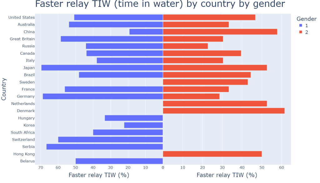
Countries are ranked from strongest swimming tradition (United States) to weakest swimming tradition (Belarus).
After a quick look at the figure above (using plotly.express), we already notice that there does not seem to be any significant positive relationship between the strength of national swimming tradition (number of meet results per country) and the percentage of faster relay TIW. Many countries with a bigger number of meet results such as the US, Australia or Great Britain have smaller faster relay TIW percentages than countries with less of a swimming tradition such as Serbia, Switzerland or Germany, and this remark can be made for both genders. One possible reason for that could be the sampling error: our data is a sample of the population (of swimmers swimming both solo and relay events at major meets) from 2015 to 2023, and perhaps that such a trend did exist before 2015. However, the difference in total observations by country between 2015 and 2023 is not a result of sampling error since our data set contains all the observations of the population for this period. In other words, the US having 121 observations and Serbia 6 between 2015 and 2023 is not a result of sampling error. Therefore we may assume that having a stronger national swimming tradition (having more athletes swimming both individual and relay events at major meets) does not correlate with the motivation of swimmers to swim faster for their country’s team based on data from 2015 to 2023, although further statistical analysis is needed to accurately confirm that (next part of the project). Some of the the data also looks fairly chaotic: a certain number of countries have a percentage of 0% for male swimmers and a much bigger pecentage for female swimmers, and vice versa. What this figure cannot tell us is whether there were any observations for these gender groups with 0% faster relay TIW, so let us have a look at the next figure to better understand all of that.
text_threshold = 7

tornado = go.Figure()
tornado.add_trace(
    go.Bar(
        x=countries_df[countries_df.index.get_level_values(1)=='1'].id_x,
        y=countries_df.index.get_level_values(0).unique(),
        name='Male total obs',
        orientation='h',
        marker_color='rgb(158,185,243)',
        xaxis='x',
    )
)
tornado.add_trace(
    go.Bar(
        x=countries_df[countries_df.index.get_level_values(1)=='2'].id_x,
        y=countries_df.index.get_level_values(0).unique(),
        name='Female total obs',
        orientation='h',
        marker_color='rgb(244,202,228)',
        xaxis='x2',
    )
)
tornado.add_trace(
    go.Bar(
        x=countries_df[countries_df.index.get_level_values(1)=='1'].fasterRelay,
        y=countries_df.index.get_level_values(0).unique(),
        name='Male faster relay',
        text=countries_df[countries_df.index.get_level_values(1)=='1'].fasterRelay_pct,
        textposition=['outside' if bar_size < text_threshold else 'inside' for bar_size in countries_df[countries_df.index.get_level_values(1)=='1'].fasterRelay],
        textfont={'family': 'Arial Black', 'size': 15},
        orientation='h',
        marker_color='blue',
        xaxis='x',
    )
)
tornado.add_trace(
    go.Bar(
        x=countries_df[countries_df.index.get_level_values(1)=='2'].fasterRelay,
        y=countries_df.index.get_level_values(0).unique(),
        name='Female faster relay',
        text=countries_df[countries_df.index.get_level_values(1)=='2'].fasterRelay_pct,
        textposition=['outside' if bar_size < text_threshold else 'inside' for bar_size in countries_df[countries_df.index.get_level_values(1)=='2'].fasterRelay],
        textfont={'family': 'Arial Black', 'size': 15},
        orientation='h',
        marker_color='red',
        xaxis='x2',
    )
)

tornado.update_layout(
    barmode='overlay',
    bargap=0.2,
    height=1000,
    width=1500,
    title={"text": "Faster relay TIW (time in water) by country by gender against total observations by country", "x": 0.5, "font": {"size": 30}},
    xaxis={"title": "Faster relay TIW (%)", "range": [70, 0], "autorange": "reversed", "domain": [0, 0.5], "title_font": {'size': 25}, "tickfont": {"size": 17}},
    xaxis2={'title': "Faster relay TIW (%)", 'domain': [0.5, 1], "title_font": {'size': 25}, "tickfont": {"size": 18}},
    yaxis={"title": "Country", "title_font": {'size': 25}, "tickfont": {"size": 18}},
    legend={'font': {'size': 20}}
)

tornado.show()
#tornado.write_image("plots/double-tornado.png")
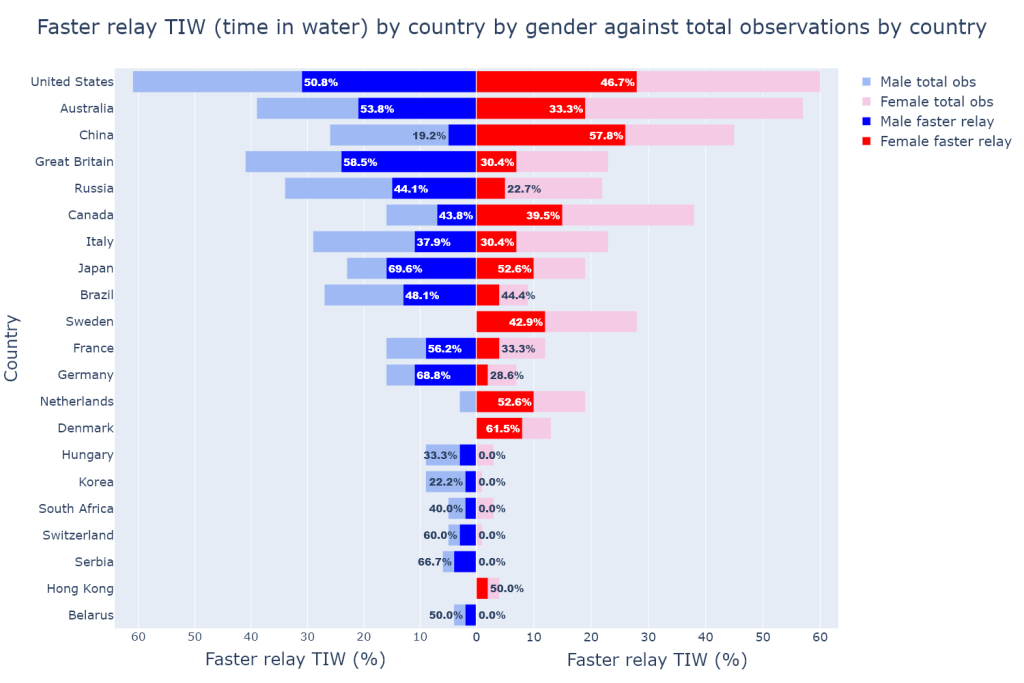
This second tornado graph shows the same data in a different way, allowing us to visualise different aspects of the data. In this figure above, interest is in showing both the number and percentage of faster relay TIW compared to the total observations by country and by gender. We notice a number of things that the previous tornado graph could not show.
Firstly, the number of observations (light blue and light red bars) by gender can vary quite a lot from country to country: whereas the United States and Italy have similar proportions of female and male swimmers, countries like Canada or Brazil have much different gender proportions, and even drastically different for countries like Sweden, the Netherlands, or Korea.
Secondly, most of the countries with a weaker swimming tradition have had more top-level male than female swimmers swim both solo and relay events at major meets. Conversely some countries with a relatively stronger swimming tradition such as Sweden or Denmark have had a much higher number of female swimmers, but strangely no top-level male swimmers representing these countries in the past 8 years. The latter observation is particularly puzzling.
From the above observations made on these two tornado graphs we may assume that the strength of a national swimming tradition seemingly does not have a significant relationship with either the percentage of faster relay TIW, or the proportions of top-level female and male swimmers representing the country at major meets.
Next, we might be curious about a potential effect of a swimmer’s age on their behaviour in relays. We are first going to group merged_df by age and then by gender, sort the data obtained and finally visualise the results with a scatter plot.
merged_df.groupby(["ageAtMeet", "gender"]).agg({"fasterRelay": pd.Series.sum, "id_x": faster_relay_pct})
# scatter plot, 2 lines per gender
| fasterRelay | id_x | ||
|---|---|---|---|
| ageAtMeet | gender | ||
| 14 | 2 | 1 | 100.0% |
| 15 | 2 | 4 | 100.0% |
| 16 | 1 | 0 | 0.0% |
| 2 | 2 | 33.3% | |
| 17 | 1 | 1 | 25.0% |
| 2 | 3 | 20.0% | |
| 18 | 1 | 3 | 42.9% |
| 2 | 11 | 50.0% | |
| 19 | 1 | 7 | 35.0% |
| 2 | 7 | 23.3% | |
| 20 | 1 | 14 | 40.0% |
| 2 | 18 | 40.0% | |
| 21 | 1 | 20 | 44.4% |
| 2 | 11 | 29.7% | |
| 22 | 1 | 21 | 38.2% |
| 2 | 18 | 45.0% | |
| 23 | 1 | 27 | 55.1% |
| 2 | 14 | 33.3% | |
| 24 | 1 | 19 | 44.2% |
| 2 | 12 | 44.4% | |
| 25 | 1 | 19 | 63.3% |
| 2 | 13 | 38.2% | |
| 26 | 1 | 15 | 57.7% |
| 2 | 12 | 48.0% | |
| 27 | 1 | 11 | 55.0% |
| 2 | 16 | 55.2% | |
| 28 | 1 | 7 | 26.9% |
| 2 | 8 | 47.1% | |
| 29 | 1 | 5 | 50.0% |
| 2 | 9 | 47.4% | |
| 30 | 1 | 6 | 54.5% |
| 2 | 1 | 33.3% | |
| 31 | 1 | 4 | 50.0% |
| 2 | 1 | 50.0% | |
| 32 | 1 | 2 | 50.0% |
| 2 | 2 | 100.0% | |
| 33 | 1 | 1 | 50.0% |
| 34 | 1 | 0 | 0.0% |
| 2 | 1 | 100.0% | |
| 37 | 1 | 0 | 0.0% |
The dataframe obtained has a 2-level MultiIndex consisting of ageAtMeet and gender values, and 2 columns being fasterRelay occurences and id_x which is the percentage of faster relays here (just like fasterRelay_pct). Since we want to check for the effect of age by gender, for each age value we want to have at least a couple observations for both female and male swimmers of that age. Right away we spot that for ageAtMeet values 14, 15, and 33 and above, there are either missing observations for certain genders or not enough observations altogether. Age 32 has only 2 female swimmer observations and the % of faster relays is 100% which when plotting the scatter graph clearly appears as an outlier (due to the small number of observations), thus we decide to exclude that age value as well since we do not consider that it does not contribute significantly to the trend. Finally, we find that the total number of observations for 16-year-old male swimmers is only 1, thus we decide to also exclude that age value. There are enough observations for the remaining age values (at least 3 for each gender) so we can go ahead and prepare the scatter plot.
print(f"16yo male obs: {merged_df[(merged_df.ageAtMeet==16) & (merged_df.gender=='1')].id_x.agg(pd.Series.count)}")
16yo male obs: 1
# the dataframe index is reset to allow for easier plotting:
age_df = merged_df[(17 <= merged_df.ageAtMeet) & (merged_df.ageAtMeet <= 31)].groupby(["ageAtMeet", "gender"]).agg({"fasterRelay": pd.Series.sum, "id_x": faster_relay_pct})
age_df = age_df.reset_index()
age_df
| ageAtMeet | gender | fasterRelay | id_x | |
|---|---|---|---|---|
| 0 | 17 | 1 | 1 | 25.0% |
| 1 | 17 | 2 | 3 | 20.0% |
| 2 | 18 | 1 | 3 | 42.9% |
| 3 | 18 | 2 | 11 | 50.0% |
| 4 | 19 | 1 | 7 | 35.0% |
| 5 | 19 | 2 | 7 | 23.3% |
| 6 | 20 | 1 | 14 | 40.0% |
| 7 | 20 | 2 | 18 | 40.0% |
| 8 | 21 | 1 | 20 | 44.4% |
| 9 | 21 | 2 | 11 | 29.7% |
| 10 | 22 | 1 | 21 | 38.2% |
| 11 | 22 | 2 | 18 | 45.0% |
| 12 | 23 | 1 | 27 | 55.1% |
| 13 | 23 | 2 | 14 | 33.3% |
| 14 | 24 | 1 | 19 | 44.2% |
| 15 | 24 | 2 | 12 | 44.4% |
| 16 | 25 | 1 | 19 | 63.3% |
| 17 | 25 | 2 | 13 | 38.2% |
| 18 | 26 | 1 | 15 | 57.7% |
| 19 | 26 | 2 | 12 | 48.0% |
| 20 | 27 | 1 | 11 | 55.0% |
| 21 | 27 | 2 | 16 | 55.2% |
| 22 | 28 | 1 | 7 | 26.9% |
| 23 | 28 | 2 | 8 | 47.1% |
| 24 | 29 | 1 | 5 | 50.0% |
| 25 | 29 | 2 | 9 | 47.4% |
| 26 | 30 | 1 | 6 | 54.5% |
| 27 | 30 | 2 | 1 | 33.3% |
| 28 | 31 | 1 | 4 | 50.0% |
| 29 | 31 | 2 | 1 | 50.0% |
age_line = px.line(x=age_df.ageAtMeet, y=age_df.id_x.str.rstrip('%').astype(float), color=age_df.gender, markers=True)
age_line.update_traces(
    name="1: Male",
    selector={'name': '1'}
)
age_line.update_traces(
    name="2: Female",
    selector={'name': '2'}
)
age_line.update_layout(
    title={"text": "Faster relay TIW (time in water) against swimmer age by gender", "x": 0.5, "font": {"size": 30}},
    height=800,
    width=1200,
    xaxis={"title": "Age (years)", "title_font": {'size': 25}, "tickfont": {"size": 17}},
    yaxis={"title": "Faster relay TIW (%)", "title_font": {'size': 25}, "tickfont": {"size": 17}},
    legend={'bordercolor': 'black', 'title': 'Gender', 'font': {'size': 20}}
)
age_line.show()
#age_line.write_image("plots/age.png")
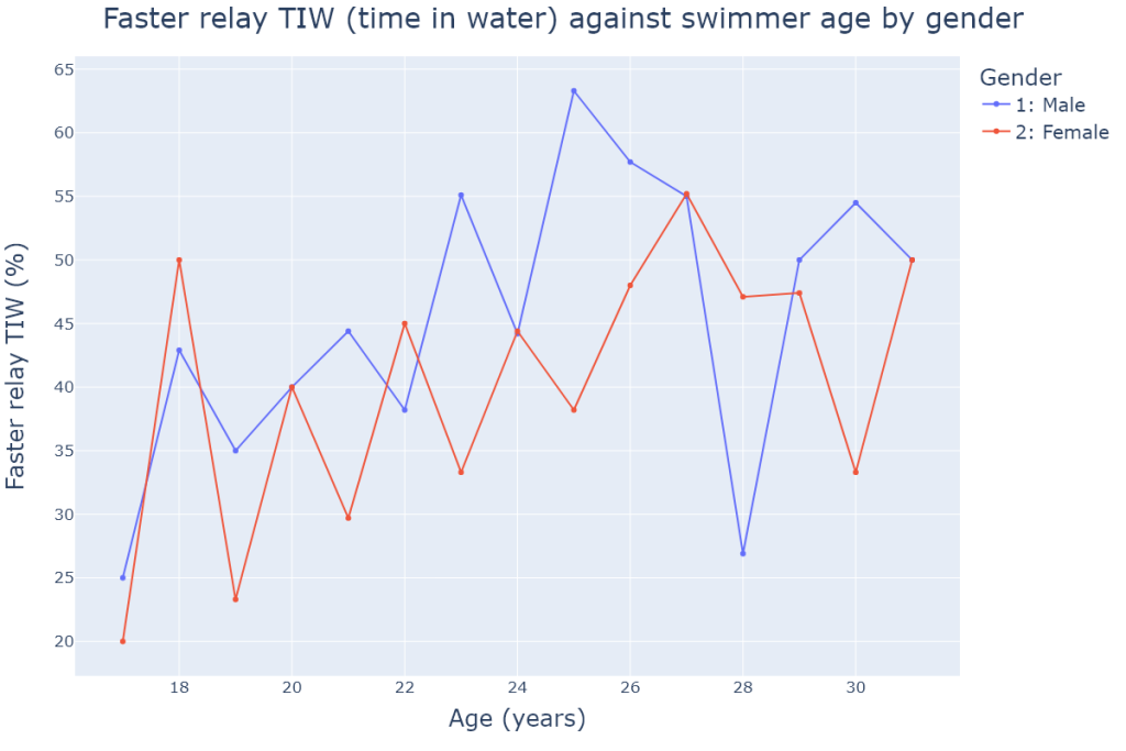
In this first simple scatter plot, we notice what looks like a positive trend for faster relay % against age for both genders. Indeed, from age 17 to age 27, the trend seems to be positive before stabilising beyond 27 years old. There are notable big spikes for female swimmers at age 18 (upward spike), and for male swimmers at age 28 (downward spike), which both significantly deviate from the assumed trend. In order to better visualise and confirm that trend, the parameter trendline is set to "lowess" (locally weighted smoothing) which enables us to better identify the trend without the noise caused by the outliers:
age_lowess = px.scatter(x=age_df.ageAtMeet, y=age_df.id_x.str.rstrip('%').astype(float), color=age_df.gender, trendline="lowess", marginal_y='box')
age_lowess.update_traces(
    name="1: Male",
    selector={'name': '1'}
)
age_lowess.update_traces(
    name="2: Female",
    selector={'name': '2'}
)
age_lowess.update_layout(
    title={"text": "Faster relay TIW (time in water) against swimmer age by gender (LOWESS)", "x": 0.5, "font": {"size": 30}},
    height=800,
    width=1300,
    xaxis={"title": "Age (years)", "title_font": {'size': 25}, "tickfont": {"size": 17}},
    yaxis={"title": "Faster relay TIW (%)", "title_font": {'size': 25}, "tickfont": {"size": 17}},
    legend={'bordercolor': 'black', 'title': 'Gender', 'font': {'size': 20}}
)
age_lowess.show()
#age_lowess.write_image("plots/age-lowess.png")
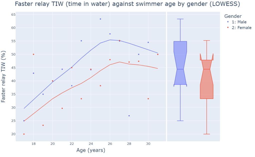
This second LOWESS scatter plot gives us a much clearer picture of the data and confirms the positive trend for both genders. What is surprising is the fact that both trends stabilise around the same age (26 years old), and the trend line of female swimmers constantly stays below that of male swimmers. Therefore we may assume that from the time they come of age until their mid-twenties, both top-level female and male swimmers become more and more motivated by swimming for their country’s team and perform better TIW in relays than in individual events more often; this trend stabilises into their late twenties for both genders. Although age seems to have the same effect on faster relay TIW for both genders, we note that after smoothing out the data, it looks like female swimmers have consistently smaller faster relay TIW percentages than male swimmers.
Looking at the marginal box plot to the right of the scatter plot, we see that the confidence intervals for the medians (the notches) of female and male swimmer groups overlap, which suggests that despite the constant gap between the two smoothed out lines, top-level female and male swimmers belong to the same population of faster relay TIW performances. Therefore we cannot conclude, for example, that top-level male swimmers are significantly more motivated by swimming relays than their female counterparts. This is an important observation.
We must keep in mind that the data points for the lowest and highest age values are less significant or have less predictive power because the number of observations is smaller.
Another factor with a potential effect on relay TIW that we might want to look at is majorMeet, from which we could extract insights on the evolution of the behaviour of swimmers over the past 8 years as well as possible differences between performances during World Championships versus during Olympic Games. Let us first group merged_df by majorMeet and then gender:
def first_item(series):
    return series.iloc[0]
meet_df = merged_df.groupby(["majorMeet", "gender"]).agg({"fasterRelay": pd.Series.sum, "id_x": faster_relay_pct, "meetYear": first_item})
for i in range(0, len(meet_df), 2):
    meet_df.at[meet_df.index[i], "avgPct"] = f"{round((float(meet_df.loc[meet_df.index[i]].id_x.rstrip('%')) + float(meet_df.loc[meet_df.index[i+1]].id_x.rstrip('%'))) / 2, 1)}%"
    meet_df.at[meet_df.index[i+1], "avgPct"] = f"{round((float(meet_df.loc[meet_df.index[i]].id_x.rstrip('%')) + float(meet_df.loc[meet_df.index[i+1]].id_x.rstrip('%'))) / 2, 1)}%"
meet_df.sort_values("meetYear", inplace=True)
meet_df
| fasterRelay | id_x | meetYear | avgPct | ||
|---|---|---|---|---|---|
| majorMeet | gender | ||||
| kazan_2015 | 1 | 29 | 50.9% | 2015 | 48.9% |
| 2 | 30 | 46.9% | 2015 | 48.9% | |
| rio_2016 | 1 | 32 | 56.1% | 2016 | 54.4% |
| 2 | 29 | 52.7% | 2016 | 54.4% | |
| budapest_2017 | 1 | 26 | 42.6% | 2017 | 40.2% |
| 2 | 22 | 37.9% | 2017 | 40.2% | |
| gwangju_2019 | 1 | 24 | 35.8% | 2019 | 37.2% |
| 2 | 22 | 38.6% | 2019 | 37.2% | |
| tokyo_2021 | 1 | 28 | 52.8% | 2021 | 48.8% |
| 2 | 26 | 44.8% | 2021 | 48.8% | |
| budapest_2022 | 1 | 17 | 35.4% | 2022 | 31.2% |
| 2 | 13 | 27.1% | 2022 | 31.2% | |
| fukuoka_2023 | 1 | 26 | 46.4% | 2023 | 41.2% |
| 2 | 22 | 36.1% | 2023 | 41.2% |
The resulting dataframe contains a 2-level MultiIndex (majorMeet and gender) and 4 columns: the dataframe was sorted by meetYear so that the majorMeet values are sorted in chronological order. The column avgPct is the average percentage of faster relay TIW and is the simple average of the faster relay TIW percentages for female and male swimmers in the same major meet (for example, for kazan_2015 the avgPct is (50.9% + 46.9%)/2 = 48.9%). We are going to plot the data as a bar chart with 2 gender bars for each major meet, and plot the OLS regression lines for World Championships and Olympic Games meets to spot potential trend differences between the two types of major meets:
# OLS line for World Championships:
X = sm.add_constant(pd.Series([1,2,3,4,5,6,7]))
model_wc = sm.OLS(pd.Series([48.9, (48.9+40.2)/2, 40.2, 37.2, (37.2+31.2)/2, 31.2, 41.2]), X).fit()
predicted_values_worlds = model_wc.predict(X)

# OLS line for Olympic Games:
X = sm.add_constant(pd.Series([1,2,3,4]))
model_oly = sm.OLS(pd.Series([54.4, 48.8+2*((54.4-48.8)/3), 48.8+((54.4-48.8)/3), 48.8]), X).fit()
predicted_values_olympics = model_oly.predict(X)
meet_histo = go.Figure()
meet_histo.add_trace(
    go.Bar(
        x = meet_df.index.get_level_values(0).unique(),
        y = meet_df[meet_df.index.get_level_values(1) == '1'].id_x.str.rstrip('%').astype(float),
        name='Male swimmers',
        marker_color='#636EFA'
    )
)
meet_histo.add_trace(
    go.Bar(
        x = meet_df.index.get_level_values(0).unique(),
        y = meet_df[meet_df.index.get_level_values(1) == '2'].id_x.str.rstrip('%').astype(float),
        name='Female swimmers',
        marker_color='#DD4477'
    )
)
meet_histo.add_trace(
    go.Scatter(
        x = meet_df.index.get_level_values(0).unique(),
        y = predicted_values_worlds,
        mode="markers",
        name="OLS - World Championships",
        marker_line_color="#2CA02C",
        marker_color='cyan'
    )
)
meet_histo.add_trace(
    go.Scatter(
        x = meet_df.index.get_level_values(0).unique()[1:5],
        y = predicted_values_olympics,
        mode="markers",
        name="OLS - Olympic Games",
        marker_line_color="rgb(166,86,40)",
        marker_color='#FFA15A'
    )
)
meet_histo.update_traces(selector={"mode": "markers"}, marker_line_width=4, marker_size=40)
world_champs = ['kazan_2015', 'budapest_2017', 'gwangju_2019', 'budapest_2022', 'fukuoka_2023']
meet_histo.add_trace(
    go.Scatter(
        x = world_champs,
        y = meet_df.loc[world_champs].avgPct.str.rstrip('%').astype(float).unique(),
        mode="markers",
        name="Avg faster relay TIW % (WC)",
        marker_color='#636EFA',
        marker_size=20,
        marker_line_color="#FC0080",
        marker_line_width=6
    )
)
meet_histo.add_annotation(text=r"$R²_{world championships}$", x=5.5, y=55, font={'size': 20}, showarrow=False)
meet_histo.add_annotation(text=f"= {model_wc.rsquared:.2f}", x=6.3, y=55, font={'size': 20}, showarrow=False)

meet_histo.update_layout(
    title={"text": "Faster relay TIW by major meet by gender", "x": 0.5, "font": {"size": 40}},
    height=900,
    width=1400,
    xaxis={"title": "Major Meet", "title_font": {'size': 25}, "tickfont": {"size": 17}, "tickangle": 45},
    yaxis={"title": "Faster relay TIW (%)", "range": [0, 65], "title_font": {'size': 25}, "tickfont": {"size": 17}},
    legend={"font": {"size": 17}},
    barmode="group",
    bargap=0.15,
    bargroupgap=0.1,
)
meet_histo.show()
#meet_histo.write_image("plots/meet-histo.png")

The figure above contains four sub-plots: a double bar chart, and two OLS (ordinary least squares) lines. The observed values fed to each OLS line are the avgPct values for their respective major meet type (Worlds or Olympics). The orange OLS line for Olympic Games is basically the line between the two avgPct values for the Rio and Tokyo Olympics since there are only two Olympic meets in our data set. The points of the cyan OLS line for World Championships are the predicted values yielded by the OLS sm.OLS() method (see code), and the red & blue points are the observed average %.
A first look at the bars tells us that there is no clear trend in the differences between male and female swimmers faster relay TIW percenteges, although we notice that in the three latest major meets (tokyo_2021, budapest_2022, fukuoka_2023 the difference between male and female percentages got bigger than in the other major meets before 2021. We also see that the bars of the two Olympic meets seem to be higher than those of the World Championships of the previous and next years; but the lack of additional data for other Olympic meets prevents us from confidently stating that athletes are truly more motivated by relays during the Olympics compared to during the Worlds.
The OLS line for World Championships allows us to better understand the trend in relay performances in World Championships, and it was computed using only the data points from World Championships meets. It is clear that from the 2015 Worlds to the most recent 2023 Worlds, there has been a downward trend in average faster relay TIW %. Although this line was plotted mainly so that the trend can be better identified at first sight, we can still take note of the R² which is .51, meaning that this simple model of fasterRelay_pct against majorMeet alone already explains 50% of the variability in relay performances of swimmers compared to solo races over the years. We can imagine that other explanatory variables could help explain the variability of relay performances, such as the evolution of swim coaching techniques, the mobility of swimmers worldwide (some swimmers train outside their home country meaning less cohesion with home team) etc. Here, based on this graph alone we can make the assumption that for the past 8 years, time itself has had a negative effect on relay TIW compared to solo TIW: top-level swimmers seem to have become less and less motivated by swimming for their country’s team in World Championships and have been increasingly swimming faster in individual events. Or perhaps swimmers are more motivated by relays when swimming in Russia and Japan than in Hungary and Korea!
Lastly, we shall check for the effect of the event categories on faster relay TIW. As a reminder, there are five solo events that have a corresponding relay leg: 100m Freestyle, 200m Freestyle, 100m Backstroke, 100m Breaststroke and 100m Butterfly. We are first going to group merged_df by event then by country, and calculate faster relay percentages:
event_country_df = merged_df.groupby(["event", "country"]).agg({"fasterRelay": pd.Series.sum, "id_x": faster_relay_pct})
event_country_df
| fasterRelay | id_x | ||
|---|---|---|---|
| event | country | ||
| 100m Backstroke | Australia | 5 | 25.0% |
| Belarus | 0 | 0.0% | |
| Brazil | 3 | 50.0% | |
| Canada | 5 | 45.5% | |
| China | 3 | 18.8% | |
| … | … | … | … |
| 200m Freestyle | Serbia | 1 | 50.0% |
| South Africa | 1 | 100.0% | |
| Sweden | 1 | 33.3% | |
| Switzerland | 2 | 100.0% | |
| United States | 18 | 69.2% |
120 rows × 2 columns
The dataframe obtained has a 2-level MultiIndex (event and country) and 2 columns, which are fasterRelay occurences and percentages. Next, we choose to exclude a list of countries and their corresponding rows from the dataframe following a threshold of at least 4 observations (rows) in the dataframe. Countries with 3 or less observations are deemed countries with too limited of a swimming tradition to significantly contribute to our results. Finally, the results are presented in a graph with 5 box plots (one for each event):
countries_to_exclude = ['Israel', 'Spain', 'Iceland', 'Greece', 'Portugal', 'Ireland', 'Austria', 'Czechia', 'Kazakhstan', 'Singapore', 'Egypt', 'Finland']
index_to_drop = []
for index, row in event_country_df.iterrows():
    if index[1] in countries_to_exclude:
        index_to_drop.append(index)

event_country_df.drop(index=index_to_drop, inplace=True)
event_country_df.reset_index(inplace=True)
event_country_median = round(event_country_df.id_x.str.rstrip('%').astype(float).median(), 1)
# event_country_mean = round(event_country_df.id_x.str.rstrip('%').astype(float).mean(), 1)
# the mean is almost equal to the median
# population_median = round(merged_df.groupby("country").agg({"id_x": faster_relay_pct}).id_x.str.rstrip('%').astype(float).median(), 1)
# --> grouping by country to find the total population median of % of faster relays is the same as calculating the % for every athlete

event_box = go.Figure()
for event in event_country_df.event.unique():
    event_box.add_trace(go.Box(y=event_country_df[event_country_df.event == event].id_x.str.rstrip('%').astype(float), name=event, boxpoints="all", notched=True, boxmean=True))
event_box.add_trace(go.Scatter(y=[event_country_median]*5, x=[event for event in event_country_df.event.unique()], mode="lines", marker_color='black', name="general median"))
event_box.update_layout(
    title={"text": "Faster relay TIW by event", "x": 0.5, "font": {"size": 40}},
    height=1100,
    width=1400,
    xaxis={"title": "Event", "title_font": {'size': 25}, "tickfont": {"size": 17}},
    yaxis={"title": "Faster relay TIW (%)", "title_font": {'size': 25}, "tickfont": {"size": 17}},
    legend={"font": {"size": 15}}
)
event_box.show()
#event_box.write_image("plots/five-boxplot.png")

The figure above contains 5 box plots corresponding to the 5 events, and the data points are every country’s percentage of faster relay TIW for each event. All data points were plotted next to the boxes, and the parameter notched was set to True which means that the 95% confidence interval of the event median is shown in the form of notches. The solid line inside the box is the median, and from the median the edges of the box spread out until the boundaries of the interval. For the 100m Breaststroke box, we see that the upper boundary of the interval is above the upper quartile which is why the box has these little legs at the top. The dashed line is the event mean.
We didn’t sample the data randomly, we deliberately retrieved data from years 2015 to 2023. So, these results should be taken with a grain of salt. The 95% confidence interval of the median basically says “if the general sample median (black line) is found within this interval then this group cannot be considered as belonging to a different population of swimmers”. However even though the sampling was not random, the distance between the 100m Freestyle median and confidence interval from the general sample median is big enough to let us assume that we have a high chance of being correct if we consider 100m Freestyle swimmers as belonging to a different population of swimmers who are significantly more motivated by swimming for their country’s team than the swimmers specialising in the other 4 events. We will be able to draw a more accurate conclusion by performing F-tests on these groups in the next part of this project.
The general sample median is contained within the confidence intervals of the 4 other events, so we can assume that they belong to the same population of relay performances. We could be tempted to say that the 200m Freestyle swimmers almost look like a significantly different group, but the general median is still within the confidence interval although very close to the lower boundary.
One last bonus graph of faster relay TIW % by relay event is plotted, which will not be extensively commented:
relay_df = merged_df.groupby(["relayEvent", "country"]).agg({"fasterRelay": pd.Series.sum, "id_x": faster_relay_pct, "gender": first_item})
index_to_drop = []
for index, row in relay_df.iterrows():
    if "Prelim" in index[0]:
        index_to_drop.append(index)
    elif index[1] in countries_to_exclude:
        index_to_drop.append(index)
relay_df.drop(index=index_to_drop, inplace=True)
relay_df.reset_index(inplace=True)
relay_df["relayName"] = [event.split("Men, ")[1].split(",\xa0\xa0Open")[0] if "Men" in event else event.split("Women, ")[1].split(",\xa0\xa0Open")[0] for event in relay_df.relayEvent]
relay_df
| relayEvent | country | fasterRelay | id_x | gender | relayName | |
|---|---|---|---|---|---|---|
| 0 | Men, 4 x 100m Freestyle, Final, Open | Australia | 4 | 100.0% | 1 | 4 x 100m Freestyle, Final |
| 1 | Men, 4 x 100m Freestyle, Final, Open | Brazil | 3 | 75.0% | 1 | 4 x 100m Freestyle, Final |
| 2 | Men, 4 x 100m Freestyle, Final, Open | Canada | 3 | 75.0% | 1 | 4 x 100m Freestyle, Final |
| 3 | Men, 4 x 100m Freestyle, Final, Open | France | 4 | 100.0% | 1 | 4 x 100m Freestyle, Final |
| 4 | Men, 4 x 100m Freestyle, Final, Open | Hungary | 2 | 100.0% | 1 | 4 x 100m Freestyle, Final |
| … | … | … | … | … | … | … |
| 64 | Women, 4 x 200m Freestyle, Final, Open | Netherlands | 1 | 25.0% | 2 | 4 x 200m Freestyle, Final |
| 65 | Women, 4 x 200m Freestyle, Final, Open | New Zealand | 0 | 0.0% | 2 | 4 x 200m Freestyle, Final |
| 66 | Women, 4 x 200m Freestyle, Final, Open | Russia | 2 | 50.0% | 2 | 4 x 200m Freestyle, Final |
| 67 | Women, 4 x 200m Freestyle, Final, Open | Sweden | 1 | 33.3% | 2 | 4 x 200m Freestyle, Final |
| 68 | Women, 4 x 200m Freestyle, Final, Open | United States | 7 | 70.0% | 2 | 4 x 200m Freestyle, Final |
69 rows × 6 columns
relay_median = relay_df.id_x.str.rstrip('%').astype(float).median()
relay_female_median = relay_df[relay_df.gender == "2"].id_x.str.rstrip('%').astype(float).median()
relay_male_median = relay_df[relay_df.gender == "1"].id_x.str.rstrip('%').astype(float).median()

relay_box = go.Figure()

yvals_1, yvals_2 = [], []
xvals_1, xvals_2 = [], []
for index, row in relay_df.iterrows():
    if row.gender == '1':
        yvals_1.append(float(row.id_x.rstrip('%')))
        xvals_1.append(row.relayName)
    elif row.gender == '2':
        yvals_2.append(float(row.id_x.rstrip('%')))
        xvals_2.append(row.relayName)


relay_box.add_trace(go.Box(x=xvals_1, y=yvals_1, name=f"Men's relays", boxpoints="all", notched=True, boxmean=True))
relay_box.add_trace(go.Box(x=xvals_2, y=yvals_2, name=f"Women's relays", boxpoints="all", notched=True, boxmean=True))

relay_box.add_trace(go.Scatter(y=[relay_median]*3, x=[relay for relay in relay_df.relayName.unique()], mode="lines", marker_color='black', name="general median"))
relay_box.add_trace(go.Scatter(y=[relay_female_median]*3, x=[relay for relay in relay_df.relayName.unique()], mode="lines", marker_color='red', name="female median"))
relay_box.add_trace(go.Scatter(y=[relay_male_median]*3, x=[relay for relay in relay_df.relayName.unique()], mode="lines", marker_color='blue', name="male median"))

relay_box.update_layout(
    title={"text": "Faster relay TIW by relay event", "x": 0.5, "font": {"size": 40}},
    height=1100,
    width=1400,
    xaxis={"title": "Relay event", "title_font": {'size': 25}, "tickfont": {"size": 17}},
    yaxis={"title": "Faster relay TIW (%)", "title_font": {'size': 25}, "tickfont": {"size": 17}},
    legend={"font": {"size": 15}},
    boxmode="group",
)
relay_box.show()
#relay_box.write_image("plots/relays-boxplot.png")
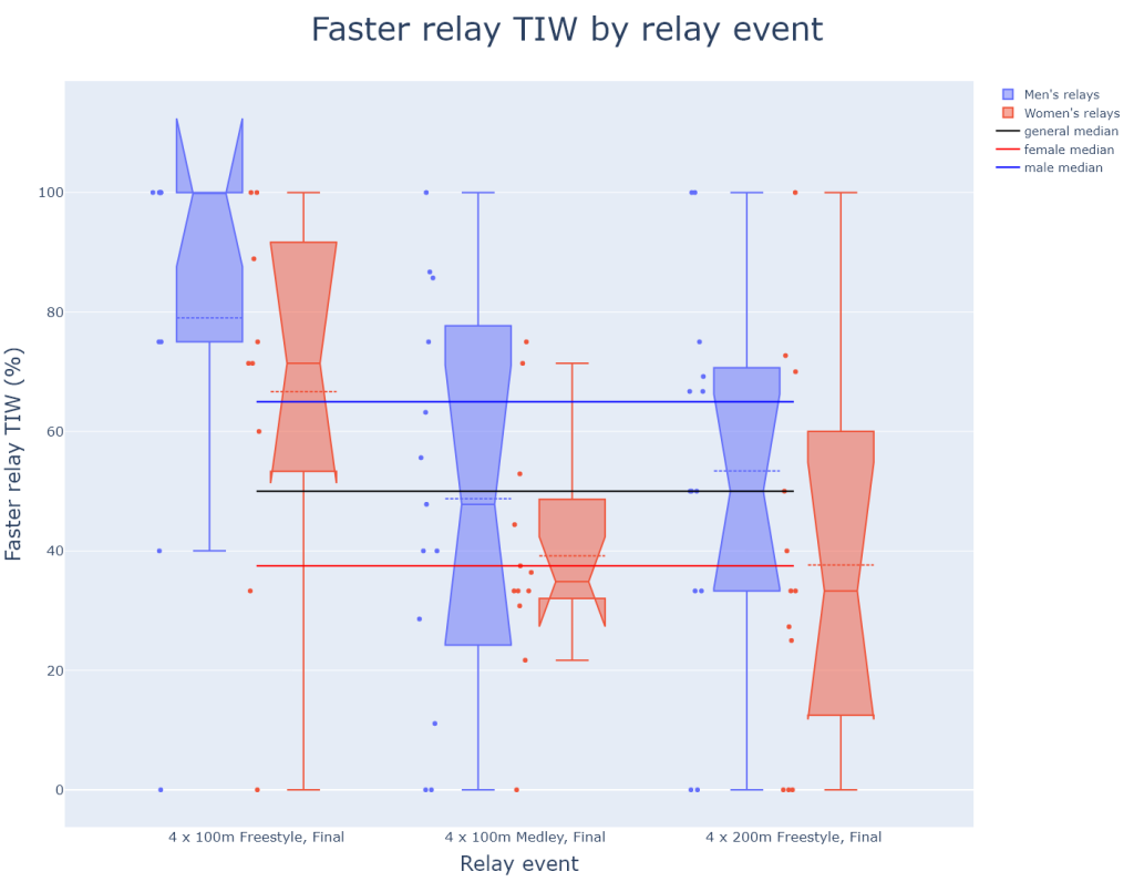
The figure above confirms the insights that the previous box plot gave us, which is that both top-level female and male freestylers can be considered as belonging to a different population of top-level swimmers who are significantly more motivated by swimming relays than individual events.
Wrapping up data visualisation
Now that we have extracted and visualised all the insights we could from the data, it is time to wrap up this section.
We studied the individual and grouped effect of gender, country, event, majorMeet and ageAtMeet on our main dependent variable fasterRelay, and from every graph we were able to extract interesting insights, and even discover the significant effects of some of those explanatory variables on fasterRelay.
We discovered that the strength of a national swimming tradition seemingly does not influence positively the dedication of swimmers to swim faster for their country’s team than in their individual races. The age of a swimmer could be positively correlated to faster relay TIW especially for young adult swimmers between 18 and 26 years old. Over the past 8 years, the number of swimmers with faster relay TIW has been trending down, especially for World Championships performances. Finally, we found that the odds are high that 100m freestyle swimmers belong to a different population of swimmers who are more motivated by swimming relays than their individual events, compared to swimmers specialising in the other four events.
EDA conclusion
The explanatory data analysis part of this project is now coming to an end, and the analysis we made of our data shed light on which of the explanatory variables from our data set could potentially help explain the variability in our dependent variable, faster relay TIW (time in water). In that sense, our analysis fulfilled the purpose of explanatory data analysis and enables us to get ahead with the third part of this project with enough confidence that a statistical model with as predictors the explanatory variables studied in this part will yield significant predictive results.
Before moving on to statistical modelling, we should bear in mind that the significance of our results in EDA as well as in the next part of the project is bound to be limited since our sampling was not random. In the first part of the project (data scraping) we captured the bulk of the population of top-level swimmers’ performances at major meets between 2015 and 2023, but could not access data for the rest of the population before that period. Had we had data for major meets before 2015, the EDA could have yielded different final results. As such, the reader should remember that the predictive power of the EDA results and the statistical models built in the next part is limited.
# exporting data for statistical modelling:
r_df = merged_df.copy()
r_df.drop(index = [index for index, row in r_df.iterrows() if row.country in countries_to_exclude], inplace=True)
r_df.relayEvent = r_df.relayEvent.str.rstrip(',\xa0\xa0Open')
r_df.to_csv("r_swim_data.csv", sep=",", columns=["swimmerId", "majorMeet", "meetYear", "event", "relayEvent", "fasterRelay", "gender", "country", "ageAtMeet"])
'Men, 4 x 100m Freestyle, Final'
Leave a Reply